
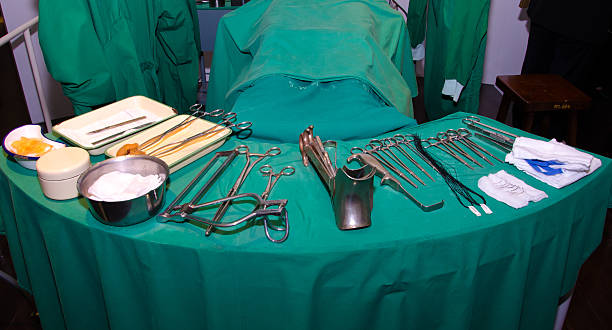
ผ่าตัด ขา กรรไกร ที่ เกาหลีมีแบบไหนบ้าง เหมือนหรือต่างกับไทยยังไง ราคาเท่าไหร่
การผ่าตัด ขา กรรไกร ที่ เกาหลีมีจุดประสงค์หลักในการแก้ไขปัญหาด้านความงาม เหมาะสำหรับคนที่มีปัญหา เช่น คางหน้ายื่นออกมายาว คางยื่นออกมา คางสั้น คางถอยกลับ ขากรรไกรกว้าง รอยยิ้มลึก ใบหน้าแบน เมื่อทำออกมาแล้วจะช่วยให้ใบหน้าได้สัดส่วนและดูเป็นธรรมชาติ…
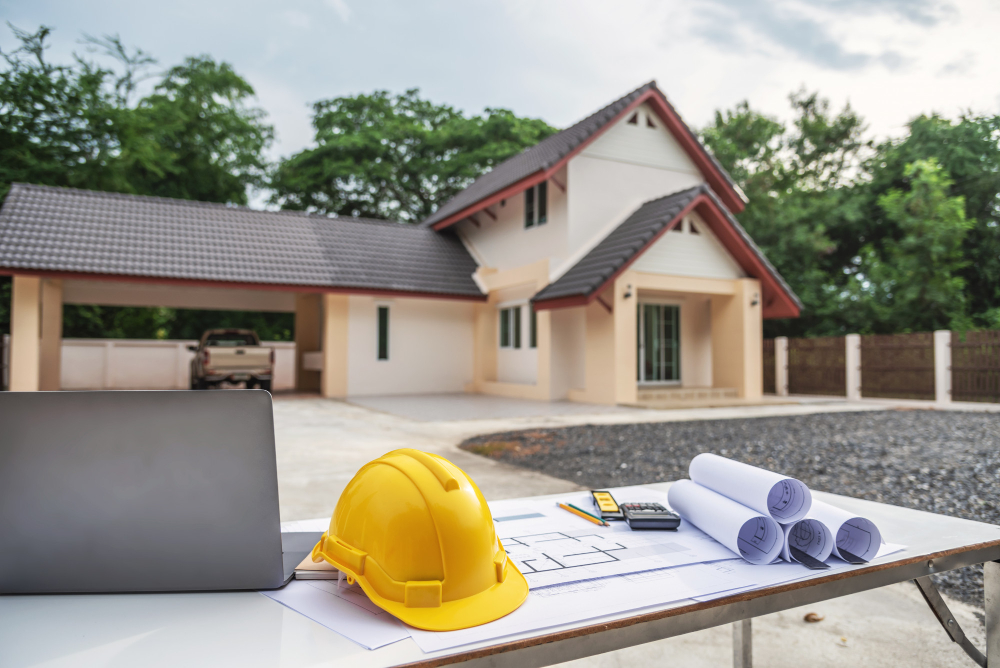
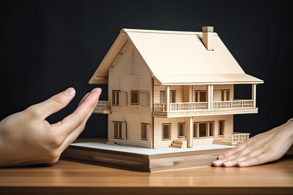
สร้างบ้านมีมาตรฐานและความสำคัญอย่างไรบ้าง
สำหรับมาตรฐานในการสร้างบ้าน ถือได้ว่าเป็นเกณฑ์ที่ใช้ในการรองรับและเปรียบเทียบในเรื่องของปริมาณและคุณภาพของการสร้างบ้าน ซึ่งสำหรับมาตรฐานในการสร้างบ้านก็จะเป็นสิ่งที่สำคัญที่สุด เพราะจะมีในเรื่องของงบประมาณที่เข้ามาเกี่ยวข้อง โดยในการสร้างบ้านท่านก็จะต้องมีการคำนึงถึงมาตรฐานในการก่อสร้าง เพราะมาตรฐานจะเป็นตัวช่วยในการกำหนดงบประมาณที่จ่ายไป เป็นตัวช่วยในการออกแบบบ้าน รวมถึงวัสดุที่มีคุณภาพ และระยะเวลาในการก่อสร้างนั่นเอง ซึ่งรับรองได้เลยว่าทุกท่านจะไม่ผิดหวังอย่างแน่นอน ถ้าหากท่านมีการเตรียมตัวในการสร้างบ้านที่ดี ท่านก็จะได้บ้านตามความต้องการที่ท่านได้วางเอาไว้อย่างแน่นอน สร้างบ้านควรมีมาตรฐานในการก่อสร้างอย่างไรบ้าง สำหรับการสร้างบ้านจะต้องมีมาตรฐานที่งานสร้างบ้านควรมี โดยจะต้องมีมาตรฐานในเรื่องของโครงสร้าง…

ผลกระทบทางเศรษฐกิจจากของพรีออเดอร์จากจีน
การใช้พรีออเดอร์จีน มีผลกระทบต่อเศรษฐกิจไทยอย่างมาก โดยเฉพาะในกลุ่มธุรกิจ SMEs ที่เป็นผู้นำการสั่งซื้อสินค้าจากจีน ซึ่งมีผลกระทบต่อธุรกิจและเศรษฐกิจในระยะยาว การสั่งซื้อสินค้าจากจีนมีความสะดวกและรวดเร็ว แต่มีความเสี่ยงทางการค้าที่สูง โดยเฉพาะเมื่อเกิดปัญหาในการส่งสินค้า การคืนเงิน หรือการส่งสินค้าที่ไม่ตรงตามความต้องการของลูกค้า ซึ่งส่งผลให้ธุรกิจต้องรับผิดชอบต่อการเสียหายทางการค้าและการเสียโอกาสในการขายสินค้าในอนาคต นอกจากนี้ การใช้ของพรีออเดอร์จากจีนยังเป็นการส่งเสริมการนำเข้าสินค้าจากต่างประเทศมากขึ้น ซึ่งส่งผลต่อการลดความสามารถในการผลิตสินค้าในประเทศ…
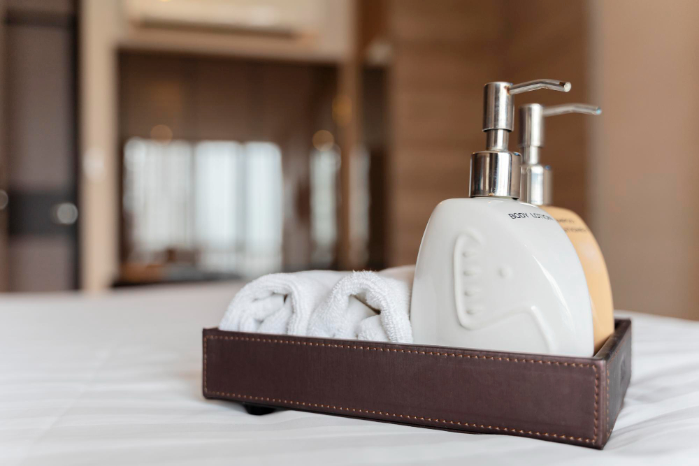
สบู่ก้อนโรงแรม ราคาส่ง ซื้อที่ไหน แนะนำสถานที่ซื้อสบู่ก้อนโรงแรมในราคาส่ง
สบู่ก้อนโรงแรมเป็นสิ่งจำเป็นในการให้บริการที่ดีและมีคุณภาพสำหรับลูกค้าโรงแรมทั่วไป สบู่ก้อนโรงแรมมีความหลากหลายในการเลือกซื้อ แต่หลายคนอาจสงสัยว่าซื้อสบู่ก้อนโรงแรมราคาส่งได้ที่ไหน หากคุณกำลังมองหาสบู่ก้อนโรงแรมราคาส่งคุณสามารถหาซื้อได้จากตัวแทนจำหน่ายสำหรับโรงแรม หรือตัวแทนจำหน่ายสำหรับธุรกิจขนาดใหญ่ ซึ่งสามารถเป็นทางเลือกที่คุ้มค่าและสะดวกสบาย คุณสามารถหาข้อมูลเพิ่มเติมเกี่ยวกับสบู่ก้อนโรงแรมราคาส่งได้จากเว็บไซต์ขายส่งออนไลน์ ซึ่งมีราคาที่ถูกกว่าร้านค้าทั่วไป แต่คุณควรตรวจสอบความน่าเชื่อถือของผู้ขายก่อนที่จะทำการสั่งซื้อ เพื่อป้องกันการซื้อสินค้าที่ไม่คุ้มค่าและไม่มีคุณภาพสูง สบู่ก้อนโรงแรม ราคาส่ง ซื้อที่ไหน แนะนำสถานที่ซื้อสบู่ก้อนโรงแรมในราคาส่ง สถานที่ซื้อ…
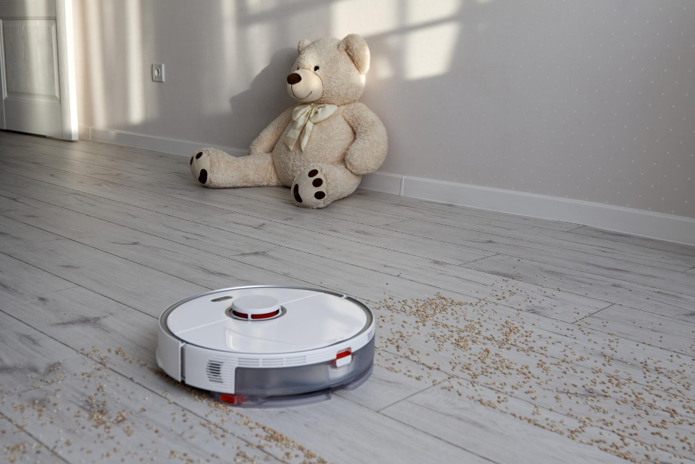
ข้อควรรู้ก่อนซื้อหุ่นยนต์ทำความสะอาด
ด้วยไลฟ์สไตล์ของมนุษย์ในปัจจุบันได้ทำให้การทำความสะอาดบ้านกลายเป็นเรื่องที่เหน็ดเหนื่อยและเสียเวลา ดังนั้นจะดีกว่าหรือไม่หากว่าคุณจะเลือกซื้อหุ่นยนต์ทำความสะอาดเอาไว้เป็นตัวช่วยสำหรับตนเองให้ได้มากที่สุดเท่าที่จะทำได้ โดยการเลือกซื้อหุ่นยนต์ทำความสะอาดมีสิ่งใดที่ต้องใส่ใจและให้ความสำคัญบ้าง รวมถึงมีข้อควรรู้อะไรบ้าง พร้อมแล้วมาดูกันเลย 1.ทุ่นแรง สำหรับหุ่นยนต์นั้นมีข้อดีก็คือช่วยทุ่นแรงได้มากกว่าเดิม ทำให้ไม่ต้องเหนื่อยกับการกวาดถูบ้าน เพราะการกวาดบ้านและถูบ้านต่างก็เป็นงานที่ต้องใช้แรงเช่นเดียวกัน หากว่าเลือกใช้หุ่นยนต์ก็รับประกันได้เลยว่าเป็นสิ่งที่เหมาะสมกับไลฟ์สไตล์คนยุคใหม่ได้ดีอย่างมาก 2.บ้านสะอาดหมดจด การที่เทคโนโลยีก้าวไปได้ไกลในยุคนี้ ทำให้การทำความสะอาดด้วยหุ่นยนต์ถือเป็นสิ่งที่จะช่วยให้บ้านสะอาดหมดจดกว่าเดิม ตอบโจทย์ได้ดีสำหรับคนที่ต้องการเลือกการทำความสะอาดอย่างมีประสิทธิภาพ และเหมาะกับคนที่เป็นโรคภูมิแพ้…

บุหรี่ไฟฟ้า ตัวช่วยเลิกบุหรี่แบบมวนดั้งเดิม ที่ตอบโจทย์มากที่สุด
สำหรับจุดขายของผู้จัดจำหน่ายบุหรี่ไฟฟ้า ก็จะเป็นการนำเสนอให้ทุกท่านเลิกสูบบุหรี่แบบมวนธรรมดา แล้วหันกลับมาสูบบุหรี่ไฟฟ้า เพราะทางการวิจัยได้มีการกล่าวไว้ว่า บุหรี่ไฟฟ้าจะมีอันตรายที่น้อยกว่าบุหรี่แบบมวน และถ้าหากผู้สูบได้เลือกที่จะสูบบุหรี่ไฟฟ้าก็จะช่วยลดการสูบบุหรี่แบบมวนได้ดีที่สุด จึงทำให้บุหรี่ไฟฟ้าเป็นอีกหนึ่งตัวเลือกสำหรับทุกท่านที่ต้องการจะเลิกการสูบบุหรี่แบบมวนธรรมดา เพราะบุหรี่ไฟฟ้าจะให้สารนิโคตินที่อยู่ในปริมาณที่เหมาะสม และส่งผลกระทบต่อร่างกายน้อยที่สุด การสูบบุหรี่ไฟฟ้าที่มีสารนิโคตินเป็นส่วนประกอบนั้น จะทำให้ผู้สูบรู้สึกอิ่มเร็ว บุหรี่ไฟฟ้าจึงได้เป็นสินค้ายอดนิยมในกลุ่มหนุ่มสาววัยรุ่นเป็นอย่างมากนั่นเอง บุหรี่ไฟฟ้า ผิดกฎหมายจริงหรือไม่ บุหรี่ไฟฟ้าถือได้ว่าเป็นสินค้าต้องห้าม…
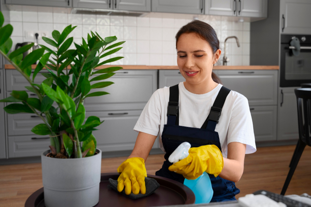
ทำไมต้องเลือกเข้ามาใช้บริการ รับทำความสะอาดบ้าน big cleaning ราคาถูก
ปัจจุบันนี้หนุ่ม สาว คนวัยทำงาน กจะไม่มีเวลา ในการทำความสะอาด หรือ ดูแลที่ยู่อาศัยของตัวเอง ดังนั้นจึงมองหาช่องทางการรับทำความสะอาดบ้าน big cleaning ราคาถูก เพื่อมาตอบสนองการดูแลที่อยู่อาศัยของตัวเอง หากคุณสนใจ หรือกำลังมองหาช่องทางสำหรับการใช้บริการทำความสะอาดเหล่านี้วันนี้ สามารถเลื่อนเข้ามาใช้บริการกับเราได้…
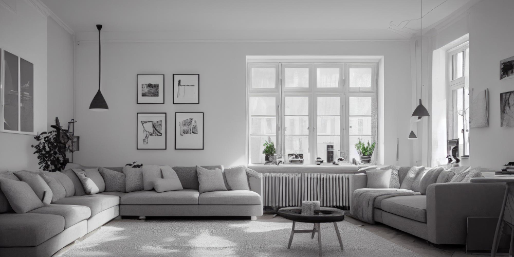
การออกแบบบ้านเดี่ยว บ้านบึง: แนวคิดและแบบแปลนที่น่าสนใจ
การออกแบบบ้านเดี่ยวเป็นหนึ่งในกระบวนการสร้างบ้านที่ต้องใช้ความคิดสร้างสรรค์และความชำนาญในการออกแบบ เพื่อให้ได้บ้านที่สวยงาม และสะดวกสบายตามความต้องการของเจ้าของบ้าน บ้านบึงเป็นหนึ่งในแบรนด์ดังที่มีชื่อเสียงในการออกแบบบ้านเดี่ยว โดยเน้นความสวยงามและความทันสมัยในการออกแบบ การออกแบบบ้านบึงมีความหลากหลายในแต่ละรุ่น โดยแต่ละรุ่นจะมีความเหมาะสมกับคนที่มีความต้องการแตกต่างกัน ตั้งแต่บ้านเล็ก แบบคอนโดมิเนียม จนถึงบ้านขนาดใหญ่ ที่มีพื้นที่ใช้สอยมากมาย โดยทุกหลังจะมีลักษณะการออกแบบที่เป็นเอกลักษณ์ของบ้านบึง ทำให้ทุกคนสามารถเลือกแบบบ้านที่ต้องการได้ตามความต้องการของตนเอง ด้วยความชำนาญและความเชี่ยวชาญในการออกแบบบ้านเดี่ยว บ้านบึงได้รับความนิยมจากลูกค้ามากมายทั้งในและต่างประเทศ…
วิธีการเลือกบริการรับบิ้วอินที่เหมาะกับคุณ
การเลือกบริการรับบิ้วอินที่เหมาะกับคุณเป็นขั้นตอนสำคัญเพื่อให้ได้บิ้วอินที่ตรงกับความต้องการและความพึงพอใจของคุณเอง ดังนั้น เรามีเคล็ดลับในการเลือกบริการรับทำบิ้วอินที่เหมาะกับคุณได้ดังนี้: 1. กำหนดวัตถุประสงค์ เริ่มต้นโดยการกำหนดวัตถุประสงค์ของการใช้บริการรับทำบิ้วอิน คุณต้องกำหนดว่าคุณต้องการบิ้วอินเพื่องานอะไร เช่น งานแต่งงาน, งานเลี้ยง, งานอีเวนต์ เป็นต้น การกำหนดวัตถุประสงค์จะช่วยคุณในการเลือกบริการที่มีความเชี่ยวชาญในงานที่คุณต้องการ ซึ่งการกำหนดวัตถุประสงค์จะช่วยให้คุณเลือกบริการรับทำบิ้วอินที่ตรงตามความต้องการของคุณ และช่วยลดเวลาในการค้นหาบริการที่ไม่เกี่ยวข้องกับความต้องการของคุณ…
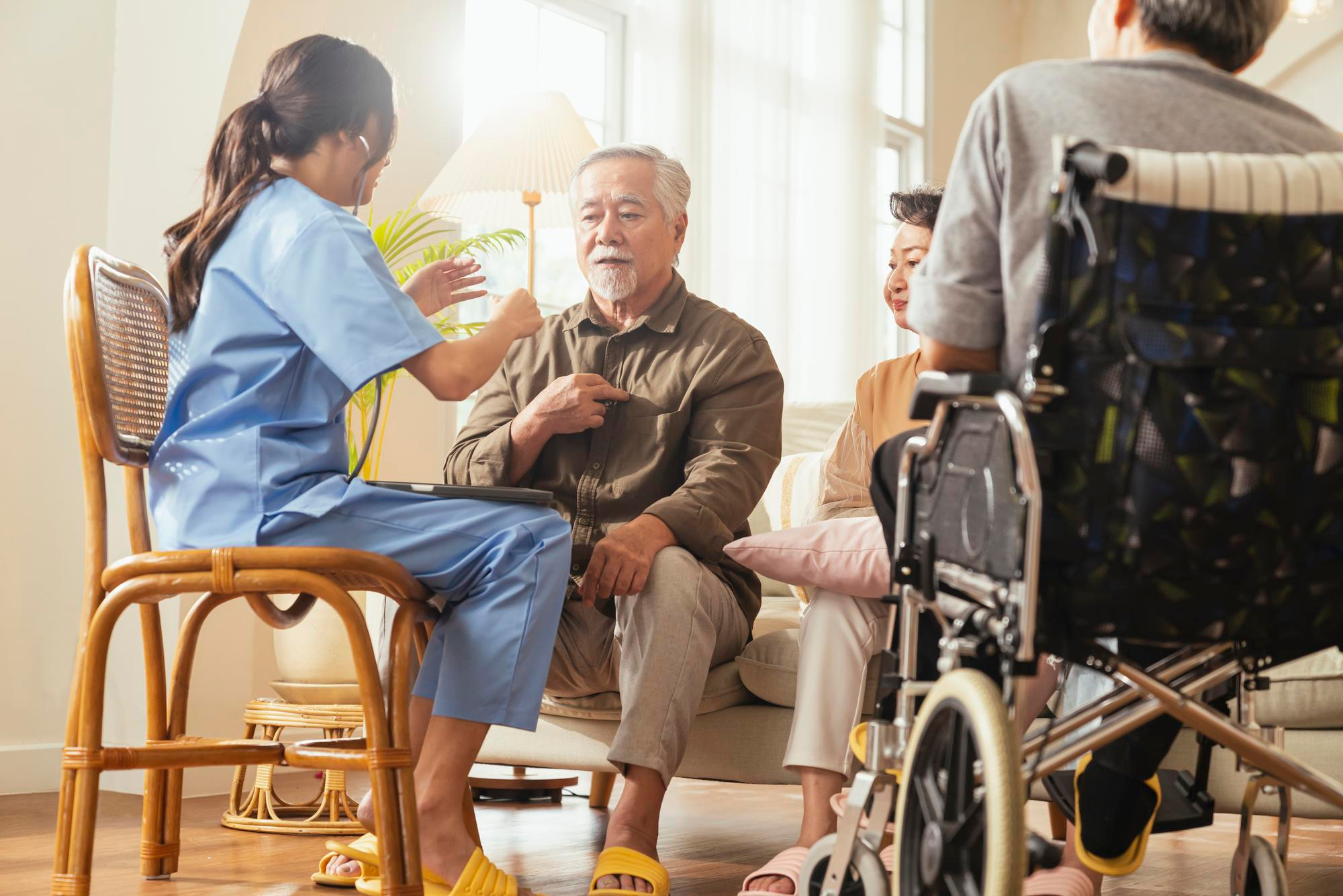
ศูนย์ฟื้นฟูกายภาพบําบัด กรุงเทพ ช่วยฟื้นฟูผู้สูงอายุได้อย่างไรบ้าง
เมื่อเข้าสู่ช่วงวัยหนึ่งของชีวิต คนเราก็จะตระหนักถึงสุขภาพร่างกายของตัวเองมากขึ้น โดยเฉพาะอย่างยิ่งในวัยชราที่ต้องได้รับการดูแลเป็นพิเศษ ซึ่งการดูแลร่างกายผู้สูงอายุนั้น นอกจากเรื่องทั่ว ๆ ไปแล้วอาจมีปัญหาหลายประการที่ต้องอาศัยผู้เชี่ยวชาญจากศูนย์ฟื้นฟูกายภาพบําบัด กรุงเทพ เข้ามาช่วยดูแลด้วย เนื่องจากสำหรับผู้สูงอายุบางท่านอาจมีภาวะที่ต้องได้รับการดูแลจากผู้เชี่ยวชาญอย่างใกล้ชิดเพื่อให้ร่างกายฟื้นฟูอย่างถูกต้องและมีประสิทธิภาพ อาการของผู้สูงอายุ ที่ควรใช้บริการศูนย์ฟื้นฟูกายภาพบําบัด กรุงเทพ ศูนย์ฟื้นฟูกายภาพบําบัด กรุงเทพ…